APR-16-2015 Magnetic Potential Energy Lab

Magnetic Potential Energy Lab

(Using physical measurements in order to derive a potential energy function)

Purpose:  The main goal here is to utilize integration calculus in order to acquire an equation which represents magnetic potential energy, and then to use that equation to verify that this system's energy is conserved.

Procedure:  We used an air track with a magnet attached to the air cart, and another magnet at the end of the track.  Increasing the angle (theta) between the air track and the horizontal, we can record varying values of the separate distance between magnets (r) caused by the magnets' repulsion of one another.  This also enables us to calculate the magnetic force at varying angles, as this force is equal to mgsin(theta), the force of gravity acting on the air-cart.  The pre-tilted apparatus is shown:

(Apparatus pre-tilt)

Values which we measured are given in the table below:

(Measured Data)

Using Newton's Laws, we can also derive how to calculate the magnetic force being applied to the air-cart.

(Magnetic force calculation)

Using this relationship, we can calculate the magnetic force at the previously recorded angles.

(Calculated Magnetic Force)

We can plot these force values against the previously recorded separation distance to form a F vs. r graph.  Using Logger Pro, we can do a curved fit of this data in order to find a function of Force as a function of r in the form of a power law.  This Logger Pro graph is shown below.

 (F vs. r)

The power law relationship is in the form of:

    F = Ar^n

From our Logger Pro curved fit data box, we can see that:

A = 0.001304

n = -1.506

Now that we've got values, we can integrate from infinity to r to obtain U(r), a function for magnetic potential energy.  This is demonstrated below:

(Magnetic Potential Energy Derivation)

We're almost ready to actually start the experiment!!!

We can input the above derived function U(r) into a new calculated column for Magnetic Potential Energy (in Logger Pro).  Once that is set up, we leveled out the track once more (no inclination).  We then began to record data via the set up Motion Sensor, all while collecting data (via calculated columns in Logger Pro) for KE, PE, and Total Energy of the system as a function of time!  This is shown below:

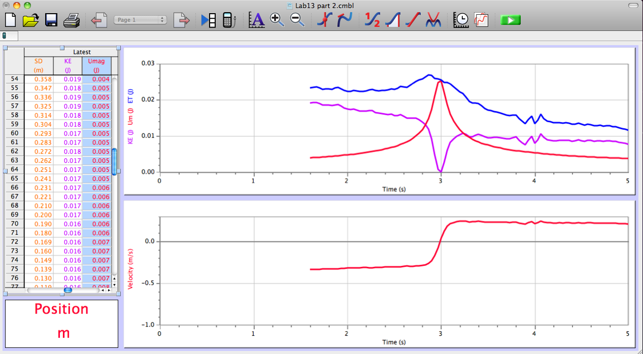
(Final Graph displaying, graphically, conservation of energy within the system)

Conclusion:  Graphically, things worked out quite pleasingly.  Using all of the data gathered, we could verify that energy was conserved within this system.  Using:

Energy(initial) = Energy(final)

KE = U(magnetic)

Sources of uncertainty in this lab include: Improperly leveled air-track, error in measuring distance (r), not calibrating phone app prior to recording angles.

MAR-23-2015 Trajectories

Trajectories

(Projectile Motion Lab)

Purpose:  To demonstrate our understanding of 2-dimensional kinematics in order to predict the impact point of a projectile (a ball) on an inclined board.

Procedure:  We first assembled the experiment apparatus.  This includes an aluminum "v-channel", steel ball, board, ring stand, clamp, paper, and carbon paper (to know where the ball strikes the floor).  Below is a complete apparatus setup.

(Apparatus on table)

Once this was set up, we used a phone app (Clinometer) in order to determine the angle between the two aluminum "v-channels".  We recorded the angle to be 28.0 degrees (+ - 0.1 degrees).  Then, we released the ball from rest at a set point on the upper "v-channel", and noticed where the projectile landed on the floor.  After seeing this, we then placed carbon paper on the floor in order to record where the projectile would hit an additional five times.

(Carbon paper being set-up in a fixed position via TAPE!!)

After we allowed the ball to drop five additional times, we recorded each mark's horizontal distance from the edge of where it left the lower "v-channel".  

 (Recording horizontal distance traveled from end of lower "v-channel")

Now we've collected all the data necessary to calculate the ball's velocity as it leaves the lower "v-channel".  Once this value is determined, we can predict where the ball should impact an inclined board as depicted below.  

(Inclined board set in place)

We recorded the horizontal distance from the end of the "v-channel" to where the ball impacted the floor to be:

Run 1:   71.4 cm

Run 2:   71.9 cm

Run 3:   72.2 cm

Run 4:   72.2 cm

Run 5:   73.0 cm

avg distance = 72.1 cm

We measured the vertical distance from the end of the "v-channel" to the floor to be:

y = 93.0 cm

Organizing this data together, we can determine the time it took the ball to hit the floor after leaving the lower "v-channel", and then use that determined time to find the value of initial horizontal velocity the ball had when leaving the "v-channel".  This work is depicted below:

(Determining initial horizontal velocity)

Now that we have the initial horizontal velocity, we can predict where on the inclined board the ball will hit, it will be some distance d.  The work to determine d is shown below.

(Determining impact distance on wooden board)

Conclusion:  Sadly, our ball was landing at approx. 0.39 m on the inclined wooden board.  Upon further investigation, I found that our initial angle measurement (between the "v-channels") had been altered, someone nudging the table or even the apparatus slightly could have caused this discrepancy.  Our theoretical calculations were all correct though!

APR-06-2015 Work-Kinetic Energy Theorem Activity

Work-Kinetic Energy Lab

(Experiment I: Work done by a non-constant spring force)

Purpose:  To use a force probe and motion sensor to determine the work done by a non-constant spring force.

Procedure:  After properly calibrating the force probe, the apparatus was assembled.  The apparatus includes a cart, track, spring, force probe, and motion sensor (shown below).  

(Complete apparatus - Motion Sensor side)

(Cart /Spring/ Force Probe side)

Using the Logger Pro software, we opened the file L11E202 (Stretching Spring) in order to obtain a force vs. position axes.  After zeroing the force probe, we began collecting data with Logger Pro.  The graph of force vs. position is shown:

(Force vs. Position)

Given the equation:

     F = kx

    k = F / x

    m = y / x = slope

The Spring Constant is the Slope of the F vs. P graph.

k = 2.956 N/m

To find the work done in STRETCHING THE SPRING, we simply integrate to find the area under this graph:

(Integration of Force vs. Position)

The Work done in Stretching the spring is:

    W = 0.1274 N*m

(Experiment II: Kinetic energy and the Work-Kinetic Energy Principle)

Procedure:  For this experiment, we will be releasing the cart from rest while the spring pulls it back.  This allows us to determine the work done BY THE SPRING, as well as the change in KE of the cart.  We first created a new calculated column within Logger Pro in order to calculate the KE of the cart at any point.  

(Graph 1 of Force (purple) vs. Position AND KE vs. Position)

(Graph 2)

What these graphs SHOULD be showing is how the work done by the spring SHOULD be equal to the KE at that point.  What these graphs DO show, is error in our calculated column for KE, and an extreme one at that.

APR-01-2015 Centripetal Force with a Motor

Centripetal Force with a Motor

Purpose:  To determine the relationship between an angle theta with the vertical and omega on a motor-driven apparatus swinging a mass connected to the apparatus via a string.

Procedure:  The apparatus was set up previously by our instructor.  It is depicted below.

(Motor-driven apparatus swinging a mass connected by a string)

A stopwatch was used in order to determine the time required for the swinging mass to make 10 complete revolutions.  This is used to determine the period T of the circular motion.  The period can then be used to calculate what omega is, this gives us our measured value of omega.

We can also calculate what omega SHOULD be by taking additional measurements, including the radius of the motion, the height of the object from the floor, and the length of the string connecting the object and the apparatus.  We can use these values, along with the application of Newton's Laws, in order to come up with a theoretical value of omega.  Firstly, in order to accomplish this, we need to express omega in terms of an angle theta.  This derivation is depicted below (along with a diagram of the apparatus and relevant measurements).

(Derivation of omega in terms of an angle theta)

We took measurements in six different instances.  In each run, we recorded the time it took the object to make 10 revolutions about it's circular path, the objects total distance (radius) from the center of the circular path it's traveling, as well as the height at which the object was relative to the ground.  Having previously measured the total height of the apparatus to be 200 cm, we can utilize the object's height relative to the ground in order to determine the angle theta being made with the vertical.

Shown below is the gathered data; values in highlighted in green are our sources of uncertainty which propagate our uncertainty in our calculated value of omega, the values highlighted in orange should be nearly equal (except they are not, due to propagated uncertainty).  The measured omega value was attained using the formula omega = (2*PI) / T     where T is the period of circular motion.

(Excel spreadsheet organizing data)

If we plot our measured value of omega versus our calculated value of omega on an xy graph, the slope SHOULD be 1.  Displayed below is my attempt to use LoggerPro on my Windows machine...

(LoggerPro graph failed attempt at linear fit)

For some reason, after naming my axis and entering values, I'm unable to have the program proceed with a linear fit.  HOWEVER, I am able to input values on a plain xy graph and the linear fit works....  This is depicted below.

(LoggerPro graph displaying slope)

We came out with a correlation of 0.9994 and slope of 1.063.  These small discrepancies are due to the propagated uncertainty in our measurements of time (from stopwatch) and our height measurements (which was taken from a 2 - meter stick).

MAR-25-2015 Centripetal Acceleration vs. Angular Frequency

Centripetal Acceleration vs. Angular Frequency

Purpose:  To determine the relationship between centripetal acceleration and angular speed.

Procedure:  For this lab, the apparatus depicted below was previously set up by the instructor.

 (Full apparatus setup)

A photogate was used to measure the length of time it takes for the disk to complete a rotation.  The apparatus was powered by electricity at varying voltages.  The acceleration was recorded via an accelerometer hooked up to LoggerPro software.  We gathered data for 10 rotations with an initial start time to to the completion of the 10th rotation t10, increasing the voltage to produce smaller rotation times and greater centripetal acceleration.  The radius of the disk was measured at approximately 13.8 cm.   

Data Gathered:  Shown below is an Excel spreadsheet containing all the data which was gathered, as well as calculated values of angular speed and values the radius should be.

(Data gathered and organized in an Excel spreadsheet)

When the measured acceleration is plotted against our calculated value of omega^2, the slope of said graph yields the radius of the disk!

(LoggerPro graph of acceleration vs. (angular speed)^2)

The slope of this line is 13.71 cm, this value for the radius of the disk matches well with our average calculated value, as well as the physically measured value.  The uncertainty in this exercise is mostly in the physically measured value of the radius of the disk, as this is an eyeball measurement, whereas all other data was collected directly and live via LoggerPro software.

MAR-16-2015 Modeling Friction Forces

Modeling Friction Forces: Part 1

(Static Friction)

Purpose:  This lab is broken into five sections, each dealing with either static or kinetic friction between the felt on the bottom of a block and the surface it's traversing.  We will be gathering data using motion sensors and force sensors for specific sections of this lab.

Procedure:  We first determined the mass of a single block (the one with the felt bottom) which we measured to be 121 g.  We then tied a string to the block, with the opposite end running over a pulley at the end of a table attached to a bent paperclip, which is in turn attached to a Styrofoam cup.  This setup is depicted below.

(Part 1 initial setup)

We then began to add small amounts of water into the cup.  This was continued until there was JUST enough water in the cup to cause the system to begin to move.  Once this occurs, we measured the mass of the cup and water to be 34 g.  

(The cup, bent paper-clip, and water combined mass JUST starts to move the system)

Next, we measured the mass of a second block, and stacked it on top of the original.  We then added more water into the cup until this new system JUST began to move.  This process was repeated until a total of four blocks were stacked upon each other.  Depicted below is a graph which contains the Normal force as the x-axis, and the force of static friction as the y-axis.

(LoggerPro linear fit graph of data collected)

The above graph shows that the slope of this line is the coefficient of static friction, and that value is 0.3712.  Below is handwritten work regarding the same data.

(Work for Part 1 of lab)

Modeling Friction Forces: Part 2

(Kinetic Friction)

Procedure:  In this section of the lab, we used a force sensor in order to determine the force of a constant pull on a block of wood traversing a surface.  First, we calibrated the force sensor using a 500 g hanging mass.  We then determined the mass of the wooden block that has felt on it's lower surface.  We held the force sensor horizontally and zeroed it.  Afterwards, we tied the force sensor and wooden block together with string.  We then used LoggerPro software to record and analyze the average force exerted on the block during a pull at constant speed.  In order to get an average force value, we used the Analyze menu in LoggerPro, then selected Statistics, then recorded the mean value of the pulling force.  This process was repeated for a total up four block stacked upon each other.  The LoggerPro graph is depicted below.

(LoggerPro linear fit graph for part 2 of lab)

It appears the above graph is incorrect in nature, as I doubt the coefficient of kinetic friction is 0.020. The data I received from a lab partner was perhaps corrupted when transferred.  The above graphs were made at home without the aid of experimental equipment.  I'll attempt to rectify this portion of the lab post-haste.

Modeling Friction Forces: Part 3

(Static Friction From A Sloped Surface)

Procedure:  We placed a block on a horizontal surface, and then raised one end of the surface until the block JUST started to slip.  At this point of maximum static friction, we recorded the angle between the horizontal and tilted surfaces.  Below is the work done to calculate the coefficient of static friction between the block and the surface it was attempting to traverse.

(Determining the coefficient of static friction)

Modeling Friction Forces: Part 4

(Kinetic Friction From Sliding A Block Down An Incline)

Procedure:  We placed a motion sensor at the top of an incline which was steep enough to cause the weighed block to accelerate downward.  Recording the angle at 20.6 degrees above the horizontal.  The physical setup as well as the solution are pictured below.

(Inclined surface at 20.6 degrees above the horizontal)

(Solution for coefficient of kinetic surface)

11-MAR-2015: Modeling the fall of an object falling with air resistance

Part 1

(Determining the relationship between air resistance force and speed)

Purpose:  The purpose of this portion of the lab is to collect data regarding the velocities of falling coffee filters and relate it to the force of air resistance acting on said coffee filters.  We will use this data and plot it appropriately in order to determine the values of k  and n in the following power-law equation:

   Fresistance = k * v^n

Procedure:  We began by walking over to the design technology building.  Inside, there is a balcony on the second floor which can be easily viewed from the nearby staircase.  We then used video capture software on our MAC systems to record the falling coffee filters (first one, then 2 stacked, up to a total of 5 stacked at a time).  Utilizing the LoggerPro software back in class, we created a reference length distance within the recorded video.  We then plotted points on the video as the object fell (at 1/30th second intervals).  Gathering all this data together, we plotted position vs. time graphs for each individual run.  An example is seen below:

(Position vs. Time graph of first run; a single coffee filter)

Having measured the mass of a single coffee filter (m = 0.00092 kg) we were able to produce a Force vs. Velocity graph.  Such graph is seen below:

(Force vs. Velocity Graph)

It is from this graph, we can see the values of k and n for our power-law equation. 

Where k = 0.01193 and n = 1.951.

Part 2

(Modeling the fall of an object including air resistance)

We gathered and organized all of our data into an Excel spreadsheet in order to determine the terminal velocity of each run (that is, a single coffee filter, to five stacked together).  

(Excel spreadsheet containing all gathered data; this section represents a single filter)

If we scroll down the velocity (v) column, we'll see that it begins to become a constant value as time goes on.  This value, is the value of terminal velocity of the coffee filter.

(Excel sheet for run 1; terminal velocity = 0.866282 m/s)

Conclusion:  To be 100% honest, this particular lab write-up is (when compared to my others) not up to standards; I was sick, as I'm sure was noticed, most of the week this lab occurred.  Therefore, my understanding of exactly what went on during this lab is, somewhat fractured.  I do understand however, the concept of how terminal velocity is represented in the Excel datasheet.